NWCSAF/GEO iSHAI
imaging Satellite
Humidity And
Instability product
Index
The name of version 2021 Clear
Air Product Processor is GEO-iSHAI (imaging Satellite Humidity And Instability). It has been developed within the NWC SAF context, aiming to
support nowcasting applications on clear air pixels.
GEO-iSHAI version 4.0.1 product aims to provide information
about water vapour and instability estimations
on clear air pixels from version 2021
supported satellites infrared channels and NWP fields. Products
are generated at high spatial and temporal resolution to support
real time meteorological applications.
The main outputs of GEO-iSHAI product are written in the iSHAI netCDF output file.
The main outputs are:
1. Total Precipitable Water (TPW): Precipitable water in layer from surface pressure to top of atmosphere.
2. Layer Precipitable Water (LPW). Corresponding to the precipitable water in three layers:
2.a BL: Precipitable water in low layer [Psurface to 850 hPa]
2.b ML: Precipitable water in middle layer [850 to 500 hPa ]
2.c HL: Precipitable water in high layer [500 hPa to top of atmosphere]
3. Stability indices: they are calculated from the retrieved profiles of temperature and humidity. The calculated indices are:
3.a Lifted Index (LI)
3.b Showalter Index (SHW)
3.c K-index (KI)
4. Skin Temperature (SKT)
5. Total Ozone (TOZ). Note: This parameter is optional and must be activated by the users and the NWP GRIB files must contains ozone fields.
6. Besides the main outputs, the differences between the above parameters calculated from the retrieved profiles of temperature and humidity (and ozone profile if activated) with the parameters calculated from the spatial, temporal and vertical interpolated profiles from background NWP are written as other outputs (following 2007 Madrid Workshop recommendation). Thus the parameters diffTPW, diffBL, diffML, diffHL, diffLI, diffSHW, diffKI, diffSKT, diffTOZ are also written in the netCDF output file.
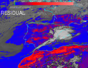
7. BT_Residual: root mean square of differences between the real bias corrected satellite and RTTOV calculated brightness temperatures on absorption channels.
Besides
the
above main output parameters, GEO-iSHAI can be optionally
configured to save input profiles, intermediate results and
retrieved profiles in
iSHAI optional binary files (writing as binary files
structures with T/q/ozone profiles together with some surface
and ancillary parameters); these files can be useful for
debugging purposes or to feed new user applications.
GEO-iSHAI products are useful in nowcasting applications, used
in synergy with other data available to the forecaster. Since
the physical basis of temperature and humidity retrieval is
based in the minimization of the error between the real bias
corrected satellite BTs and the synthetic BTs calculated from
the profiles and taking into account the limited number of
channels and the spectral information of the supported NWC/GEO
imager satellite instruments, GEO-iSHAI mainly improve the
humidity profiles of the background NWP in middle and high
levels. Despite of this, the retrieved fields have a higher
spatial resolution compared with the forecast. This fact must be
taken into account by the users when the GEO-iSHAI outputs are
used in nowcasting applications.
These web pages contain practical information on the use and
configuration of GEO-iSHAI. The content has been extracted from
the User Manual of GEO-iSHAI version v4.0.1 included in the
NWC/GEO software package release 2021 (it is also valid for
version 2018.1). Current documentation can be found at the NWC
SAF Helpdesk web: http://nwc-saf.eumetsat.int.
In the References
are also provided the URL links to the version 2021 documentation.
It describes the
characteristics, how to configure and how to execute the GEO-iSHAI
processor; including the needed input files and the resulting
outputs. A summary of definitions, acronyms and abbreviations can
be seen here.
Summary
of iSHAI algorithm
The iSHAI algorithm is composed of a statistical retrieval
followed by a physical retrieval of temperature and moisture
profiles using infrared (IR) brightness temperatures (BTs)
measured by GEO imager satellites and a background NWP forecast
as main inputs. It has two main steps.
In the first step, the iSHAI First Guess profile is built using a set of non-linear regressions from collocated background NWP temperature and humidity profiles and real satellite bias corrected BTs.
In the second step, a physical retrieval algorithm (optimal estimation) is applied with some improvements over the classical approach. The improvements over the classical approach are: a) the use of EOFs to reduce the dimension of matrix and reduce the computation time (2 EOFs for T, 3 EOFs for q and 1 EOF for Tskin) and b) a regularization parameter.
The second step is only executed if the distance (BT_RMS) between satellite bias corrected BTs and synthetic BTRTTOV
(BTs calculated using RTTOV from
FG profile) on the non-window channels is greater than a
configurable threshold (BT_RMS_THRESHOLD).
Note: WV6.2, WV7.3 and IR13.4 in SEVIRI case
and WV6.2, WV6.9, WV7.3 and IR13.3 in AHI or ABI case.
The Cloud Mask output is used to identify clear air
pixels. Only if the pixel is labelled as clear air and the
satellite zenith angle of this pixel lies within the configurable
threshold (default 70º ), the
processing is made.
A more detailed description of iSHAI algorithm is made here. Full details of the algorithm can be found in "Algorithm Theoretical Basis Document for iSHAI Product” and in the “User Manual for the Clear Air Product Processor of the NWC/GEO: Science Part” document.
GEO-iSHAI
algorithm remains based in Jun Li’s algorithm for legacy GOES
Sounder physical retrieval algorithm (physical iterative
approach with non-linear regression as first guess) but adapted
for RTTOV and the supported GEO imager satellites. Jun Li
(CIMSS-Wisconsin) algorithm is also the proposed as Day-1
algorithm for the GOES-R processing by NOAA (Li, 2010).
GEO-iSHAI releases 2021 and 2018.1 has some major updates with
respect to former version 2016. The summary of changes with
respect to former version can be read here.
There are two kind of outputs:
The main outputs provided are parameters informing about the water vapour content in the vertical column (total and in selected layers) and about the atmospheric thermal instability. These parameters are computed using the final retrieved temperature and humidity profiles.
Also the Skin Temperature (SKT) and Total Ozone (TOZ) are additional outputs.
As additional outputs, GEO-iSHAI also provides the differences between the above parameters, computed from the final retrieved profiles, and similar ones computed from the forecasted background profiles. These deviations are important for
(1) signalling areas with discrepancies between model forecast and the observations
(2) showing the added value of GEO imagers satellite observations.
The fields are now data fields only on clear pixels written as integer scaled fields. The NWCGEO netCDF has been designed in order to be standard. Thus, iSHAI netCDF files can be used with free and standard meteorological tools. As an example, all the iSHAI images in this web pages have been generated with the free and interactive McIDAS-V tool. Then, any user could use its own tools or use these free and standard meteorological tools to exploit iSHAI and NWCGEO netCDF files.
Optionally, GEO-iSHAI can be configured to keep the final retrieved profiles and the intermediate profiles. This allows users:
(1) to feed new applications or to compute specific stability indices at their own
(2) to debug and test their installation
(3) monitor GEO-iSHAI performances
(4) convert to standard formats in order to use for 3D use.
Since GEO-iSHAI is executed locally by the users, the collocated temperature, specific humidity and ozone profiles with satellite data can be written in optional binary files at different steps of the algorithm. The main advantage to get spatial, temporal and vertically collocated (T, q, ozone) profiles with satellite data is to allow debugging activities or generating new parameters or stability indices or generation of 3D displays as vertical cross sections or 3D visualizations or generation of validation datasets. These applications are only a few among other applications that could be used.
Examples of the use of optional iSHAI binary files outputs with 3D tools can be seen below in visualization example chapter. More examples on the use of the GEO-iSHAI and former PGE13 SPhR binary file in nowcasting can be found in the References.
Examples on how to use the GEO-iSHAI binary files to generate validation dataset can be found in the Validation Report.
In this section a description of the inputs, coefficients files content and user configurable parameters is made.
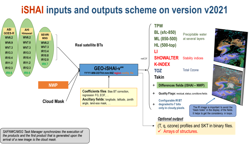
The inputs and outputs scheme is shown in the Figure below. A more detatailed explanation of the implementation and execution steps can be found here.
Figure 1: GEO-iSHAI inputs and outputs scheme
A region configuration file and a GEO-iSHAI model configuration file (with the diverse parameters and options that are indicated by the user for calculation, are needed as mandatory parameters in order to execute the GEO-iSHAI command.
GEO-iSHAI has been designed in a highly modular manner and allows a user selectable configuration.
The user configurable parameters are determined through the GEO-iSHAI model configuration file. It is the third argument required by the GEO-iSHAI program. Thus, to change the configuration used to execute the GEO-iSHAI code is as easy as changing the third argument when the GEO-iSHAI is run. A more detailed description of the iSHAI configurable parameters can be found here.
Thus, the user can have several GEO-iSHAI model configurations files in the $SAFNWC/config and GEO-iSHAI can be executed on real time with different configurations depending on the region to process, the hour of the image, etc. As an example, users can execute GEO-iSHAI on the full disk with a large FOR width and with only one iteration step or, on the other side, to execute GEO-iSHAI over a small region centred in the area of interest with small FOR width and with up to three iterations.
Also users could choose between P or HYB mode using the keyword NWP_EXEC_MODE
The main inputs are: satellite data, NWP data, a Cloud Mask for the region to process and some ancillary data. More detailed description is available here.
Concerning the coefficients files a list and a description is available here; more specific scientific information about theoretical aspects can be found in the GEO-iSHAI Algorithm Theoretical Basis Document.
A list of GEO-iSHAI Product Assumptions and Limitations can be seen here.
Graphic displays of GEO-iSHAI product parameters generated at the AEMET NWCSAF/MSG Reference System area are available on real-time in the web site of the NWC SAF Help Desk (http://www.nwcsaf.org).
For the display of the clear air outputs, a set of colour enhancement tables similar to the ones used by CIMSS for the visualisation of the GOES derived TPW and LI products has been selected.
In releases 2021 and 2018.1, the format of the file is netCDF and GEO-iSHAI outputs are not image like fields and they are data fields; this has the advantage to allow use in calculations of derived fields as temporal trends and spatial gradients.Because of this, it is the responsibility of the user to use adequate tools to generate images similar to the ones in previous versions.
Among others, there are some free available tools as McIDAS-V or IDV or HDF-View that can do this using just the GEO-iSHAI netCDF files.
As commented in the iSHAI
outputs description, to complete the image on cloudy pixels and
avoid black holes in the iSHAI images the BT from one configurable
IR BT channel has been added to GEO-iSHAI netCDF file. BTs from
the configurable IR channel have been scaled in order to store it
in 7 pixels, after scaling, and the values are written in the
range [0-127] only in cloudy pixels determined by the cloud mask
(GEO-CMA product). This field could be later used to generate
adequate images in which cloudy pixels are grey scaled and clear
pixels are colour scaled. By default is configured the cleanest IR
window channel in each satellite (In the MSG
(SEVIRI) case the default channel is the IR10.8 channel. In
the Himawari (AHI) or GOES-R class case the it the IR channel
in the 10.4 μm region).
As one example, the process with a generic tool to generate an image as the ones shown in iSHAI images could be the following:
open the netCDF file
read or click over a field parameter
adjust the range and assign a color palette
read or click the scaled BT from configurable IR channel to be displayed on the black holes of cloudy pixels.
In the case of McIDAS-V, the mechanism to represent in a color palette the clear air pixels, and as grey, the cloudy pixels is based in to using a color palette for the parameters shown on clear pixels and to use a gray color palette on cloudy pixels and all pixels where the value is equal to missing code are considered transparent.
In other tools a mechanism to generate separately the clear and cloudy images with different value ranges and fixing to a reserved low value, the missing data value and combine it using a combined color palette with color for clear air range value and grey for cloudy range value could be needed.
Also it is possible to
generate separated images for iSHAI fields and for the IR band
(using a grey color palette) and later use programs like
ImageMagick to declare as transparent the black or white pixels in
the iSHAI images and make a composition of the transparent iSHAI
images over the grey IR band image.
Example
of MSG satellite visualization
In the Figures below, the images corresponding to the case study of 10th August 2016 at 12UTC using MSG-3 satellite are shown as an example. The images have been generated with GEO-iSHAI v4.0 algorithm netCDF files and McIDAS-V. The images have been reprocessed using:
GEO-iSHAI v4.0 with the 2018.1 version
pixel by pixel FOR
forcing one iteration of the physical retrieval step in all pixels
using ECMWF hybrid GRIB files every hour from t+00 to t+24 of the 00UTC run from 10th August 2016.
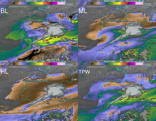
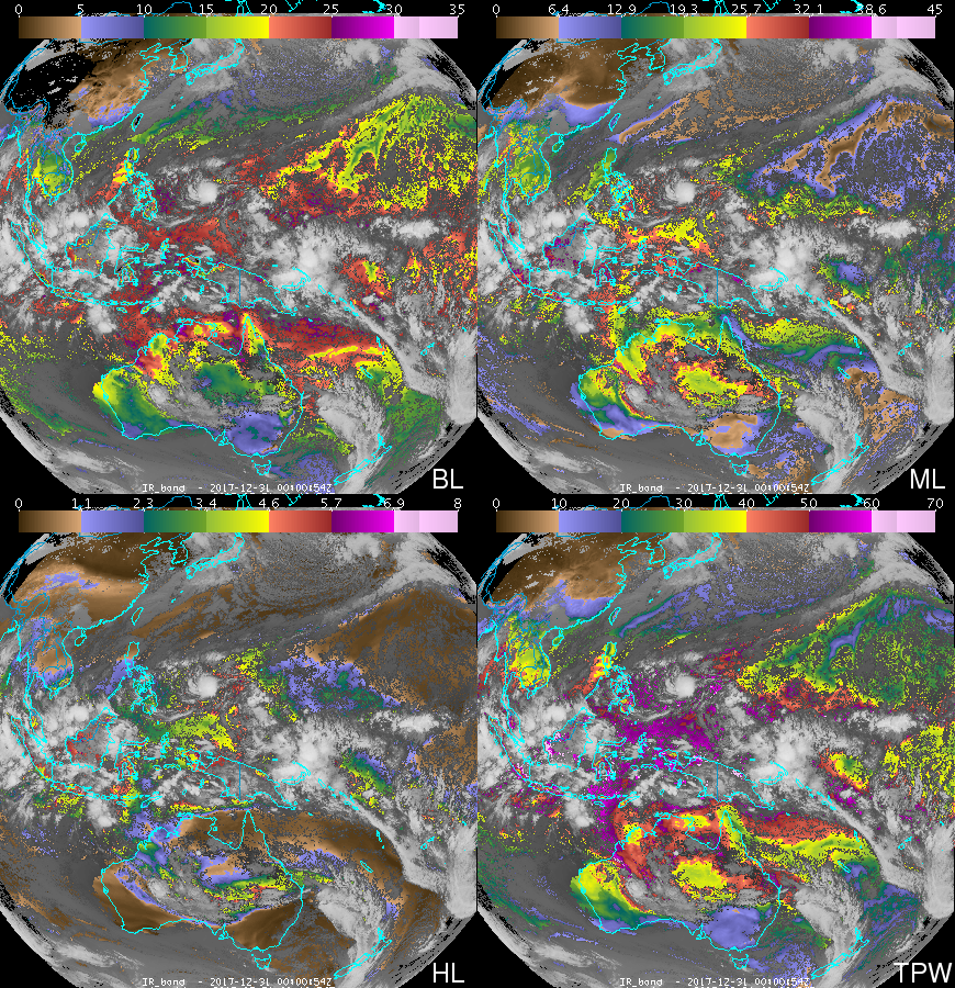
Example of GEO-iSHAI BL, ML, HL and TPW from 12 UTC on 10
August 2016 produced from SEVIRI on MSG-3.
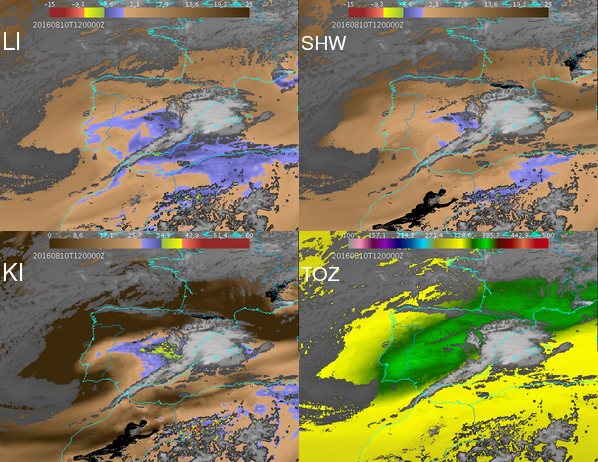
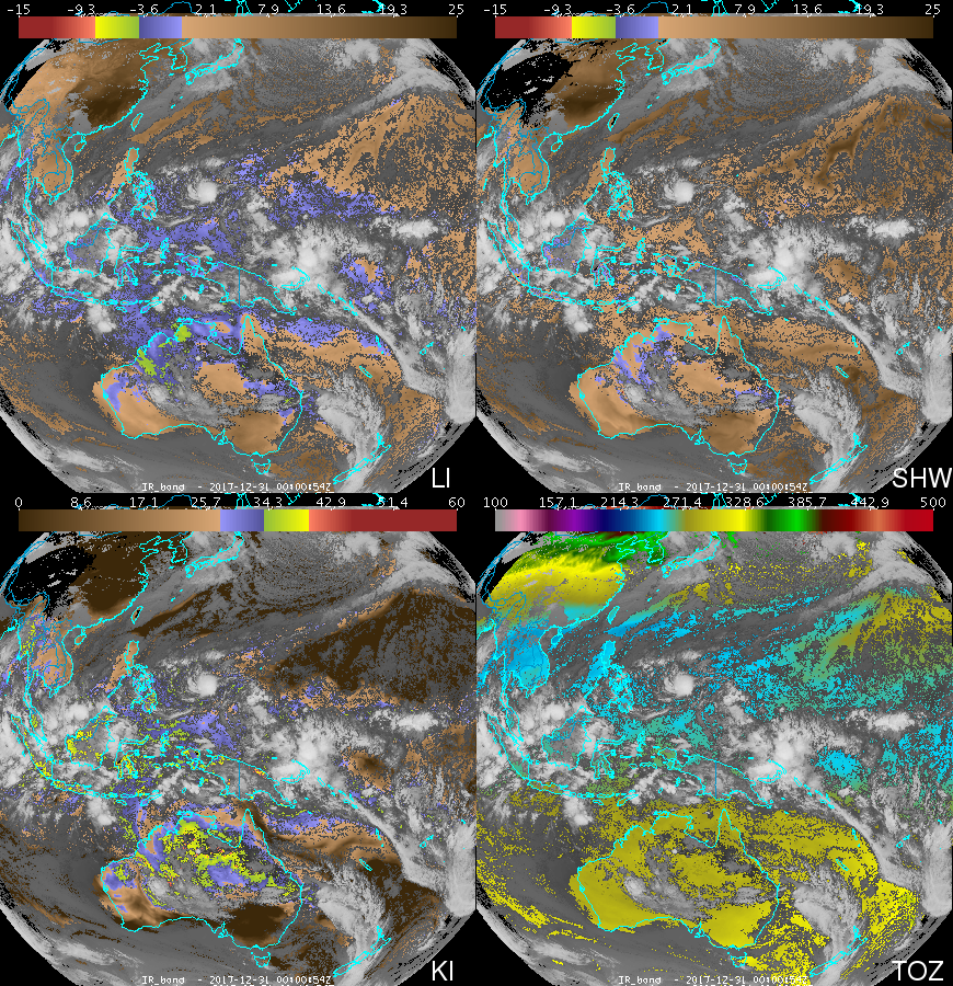
Example GEO-iSHAI LI, SHW, KI and TOZ from 12Z 10 August
2016 produced from MSG-3.
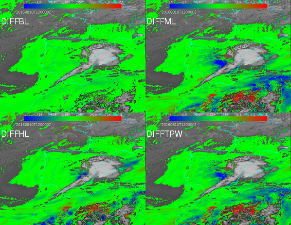
Example GEO-iSHAI diffBL, diffML, diffHL and diffTPW
from 12z on 10 August 2016 produced from MSG-3.
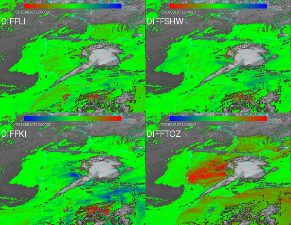
Example of GEO-iSHAI diffLI, diffSHW,diffKI and diffTOZ
from 12 UTC on 10 August 2016 produced from MSG-3.
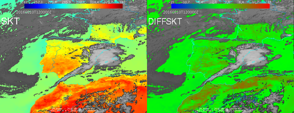
Example of GEO-iSHAI SKT and diffSKT 12 UTC on 10 August
2016 produced from MSG-3.
Example of GEO-iSHAI diffLI, diffSHW,diffKI and diffTOZ
from 12 UTC on 10 August 2016 produced from MSG-3.
One of the best
ways to exploit the water vapour and the stability indices
generated by GEO-iSHAI software is to take advantage of the high
spatial and temporal resolution of SEVIRI and to use loops of
images to monitor their evolution. See a summary of
the images and loops for the case study of 10th
August 2016.
More case studies:
a) case study 1st of
May 2019
b) case study 8th of July
2019
c) case study 22th of July
2019
Example
of Himawari satellite visualization
In the Figures below, the images corresponding to the 31 December 2017 at 12UTC from AHI instrument on Himawari-8 are shown as an example. The images have been generated with GEO-iSHAI v4.0 algorithm netCDF files and McIDAS-V.
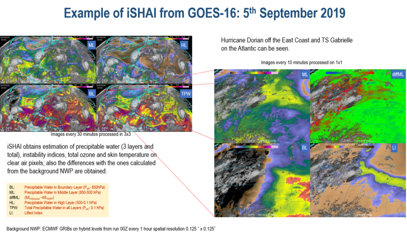
The loop of the
images corresponding to the 5th September 2019 from
ABI instrument on GOES-16 is available clicking in the Figure below or on this link. iSHAI
outputs of Hurricane Dorian off the Carolinas coasts and TS
Gabrielle on the Atlantic can be seen. Also a zoom on the Rocky
mountains can be seen.
More case studies will be incorporated in the NWCSAF web server.
Synthetic images of
MTG-FCI and IASI as proxy of MTG-IRS has been generated using
the AEMET PGE00 tool.
In this link are available some examples:
AEMET's PGE00 tool mades the made the collocation of ECMWF profiles from GRIB files on hybrid levels to call RTTOV to calculate reflectances on VIS and NIR channels and BTs on IR channels of MTG-FCI on clear and cloudy conditions. The outputs could be used to:
a) new MTG-FCI RGBs. As example synthetic MTG-FCI true color and natural RGBs are shown.
b)
Investigate the possibilities of new products to estimate
precipitable water using the new VIS and NIR channels.
As example are shown the estimations of TPW using VIS0.9 microns
channels and the estimation of HL (precipitable water in High
Layer)
c) Evolution of iSHAI for
MTG-FCI. At this moment the FG regression
coefficients for MTG-FCI are available and it will be tested with
synthetic MTG-FCI BTs soon.
AEMET's PGE00 tool
mades the made the collocation of ECMWF profiles from GRIB files
on hybrid levels to call RTTOV to calculate IASI spectra on
clear and cloudy conditions.
A loop of IASI
synthetic BTs from 13 slots every 30 minutes on MSG projection
is available in the above link for
the region of MTG-IRS dwell. It can be compared with MTG-FCI
channels.
Soon it will
repeated using MTG-FCI on future MTG-FCI grid (nominal
resolution 2 km x2 km) and MTG-IRS in a grid of 4 km x 4km ( at
1 out 2 x 1 out 2 MTG-FCI pixels).
A list of references is provided here.