
Automatic Satellite Image Interpretation-Tropopause Folding
NWCSAF/GEO v2021
Table of contents
1. Goal of the ASII-NG products
2. ASII-TF algorithm summary description
3. List of inputs for ASII-TF
4. Coverage and resolution
5. Description of ASII-TF output
6. Example of ASII-TF visualisation
Access to "Algorithm Theoretical Basis Document for the "Automatic Satellite Image Interpretation - Next Generation" Processor of the NWC/GEO" for a more detailed description.
1. Goal of the ASII-NG products
ASII-NG aims at detecting atmospheric features which are of interest to meteorologists and other users. In contrast to the ASII product (further development is frozen), where the focus was on identification of conceptual models, the ASII-NG product in its current stage is clearly linked to Clear Air Turbulence (CAT), which makes it relevant for meteorologists and aviation end users.
Clear-air turbulence is generally non-convective turbulence outside the planetary boundary layer, often in the upper troposphere. CAT typically has a patchy structure and horizontal dimensions of 80-500 km in the along-wind direction and 20-100 km in the across-wind direction. Vertical dimensions are 500-1000 m, and the lifespan of CAT is between half an hour and a day (Overeem 2002). As CAT involves physical processes with scales usually smaller than the resolution of numerical weather prediction (NWP) models, forecasts of CAT with NWP are difficult to perform. Therefore, it is of interest to identify areas with risk of CAT from satellite observations. Common causes and sources of CAT are:
- Tropopause folds
- Gravity waves (e.g. mountain waves)
- Air mass boundaries (e.g. fronts)
- Wind shear (e.g. jet streams)
- Thunderstorm complexes
At this stage, the feature detection covers the first two phenomena in two separate sub-products, ASII-TF for tropopause foldings and ASII-GW for gravity waves.
2. ASII-TF algorithm summary description
A tropopause fold describes the downward intrusion of stratospheric air into the troposphere which results in a folding of the tropopause, as schematically illustrated in Figure 1. Typically at a tropopause fold there is the vertical shearing at the jet stream combined with the ageostrophic convergence of polar, subtropical, and stratospheric air masses. Tropopause folds mark the change in the height of the tropopause and are characterized by the occurrence of strong turbulence. Stratospheric air, which characteristically has a low moisture content and a high potential vorticity can protrude down to the mid or even the lower troposphere. Consequently, tropopause folds can be located by their association with gradients in upper level moisture, which are evident in the WV 6.2 µm channel sensitive to upper tropospheric water vapour. The tropopause height can be estimated from NWP parameters such as temperature, specific humidity or potential vorticity. Additionally, the ozone content derived from the IR channel at 9.7 µm is a good indicator for the presence of a tropopause fold: the lower the tropopause the more ozone is sensed by the instrument.
To derive the probability of a tropopause fold, a logistic regression relation is applied (input parameters given in section 3).
Note: v2021 has been adapted to HIMAWARI and GOES-R sensors whose channels partly have somewhat different central wavelengths. For the sake of readability, the text simply refers to the SEVIRI characteristics.
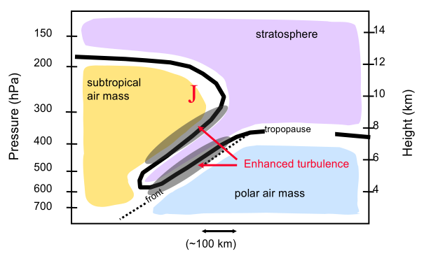
Figure 1: Illustration of a tropopause fold. (© Feltz and Wimmers 2010)
3. List of inputs for ASII-TF
Table 1 shows the input parameters required for the detection of tropopause folds. Based on specific humidity, the height of the tropopause [hPa] is calculated from the NWP data. It is the gradient field that serves as input into the logistic regression. It is recommended that NWP data be provided up to the 50 hPa level to ensure that the tropopause is captured. Brightness temperatures from channel WV 6.2 µm directly serve as input, yet there are also some post-processed satellite data involved: From WV 6.2 µm, also the gradient is input; moreover, the dark-stripe detection described in Jann (2002) is applied to a somewhat smoothed version of the field, and it is the distance from the stripe edge that serves as one of the predictors. The channel difference IR 9.7 µm – IR 10.8 µm enters the logistic regression relation in form of its gradient field.
Table 1: Input to logistic regression for tropopause folds
| NWP parameter | Satellite data |
| specific humidity | WV 6.2 µm |
| wind speed at 300 hPa | IR 9.7 µm |
| shear vorticity at 300 hPa | IR 10.8 µm |
4. Coverage and resolution
- The product is extracted in full image resolution using the satellite projection.
- The region for processing is user-defined.
5. Description of ASII-TF output
The ASII-TF product is encoded in a standard NWCSAF netCDF output file. Apart from the standard fields, the netCDF file holds the derived probability for occurrence of tropopause folding. For each pixel a value between 0 and 100% is assigned. Additionally, status flags are provided to give details on processing issues.
6. Example of ASII-TF visualisation
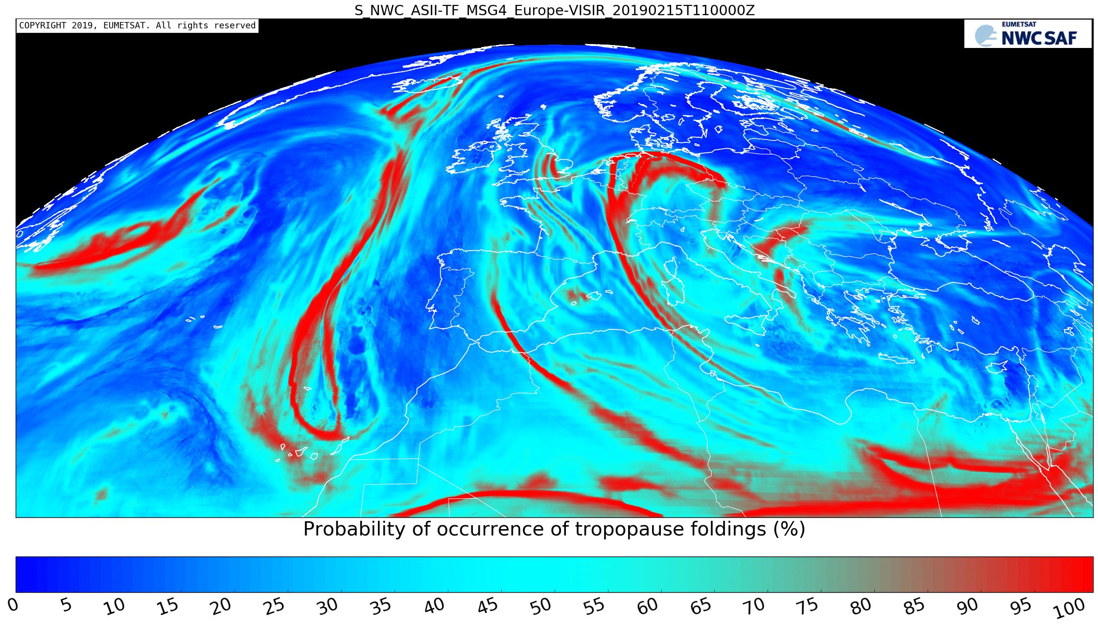
Figure 2: ASII-TF probability of tropopause fold (highest probabilities in red).