
|
| Automatic Satellite Image Interpretation |
1. Goal of the ASII product
The Automatic Satellite Image Interpretation product (ASII) aims at interpreting the SEVIRI satellite image data in terms of conceptual models (CM). CMs combine physical atmospheric processes as described in NWP model data with corresponding typical cloud features in satellite imagery. A CM diagnosis can be used for synoptic analyses and provides a deeper understanding of ongoing atmospheric processes. Further on, it can also be used to determine the stages of development of ongoing meteorological processes.
PGE10 carries out the recognition of CMs in two different modes:
- ASII: Uses MSG SEVIRI image data alone to provide the CM analysis
- ASIINWP: Additionally exploits NWP data
2. ASII algorithm summary description
Basic concept
The product generation uses pattern recognition methods and extracts fundamental information related to the shape of the cloud feature and their respective position in context to other cloud features. Implemented pattern recognition methods are:
- Detection of frontal areas
- Detection of S-shaped lines
- Detection of circular-shaped cells
- Detection of black stripes in WV images
- Detection of narrow cloud fibres
- Detection of curvature direction
- Detection of spiral cloud structures
For a detailed description of the different pattern recognition methods used for each CM see the relevant chapters in the User Manual.
| Conceptual model | Chapter in the User Manual |
| Cold front | 2.3.1.1 |
| Cold front in warm air advection | 2.3.1.1 |
| Warm front | 2.3.1.2 |
| Occlusion | 2.3.1.3 |
| Wave | 2.3.1.4 |
| Developing wave | 2.3.1.4 |
| Upper wave | 2.3.1.5 |
| Front intensification by jet | 2.3.1.6 |
| Dry intrusion | 2.3.1.7 |
| Upper level low | 2.3.1.8 |
| Comma cloud | 2.3.1.9 |
| Enhanced cumulus | 2.3.1.10 |
| Cumulonimbus | 2.3.1.11 |
| Mesoscale convective system | 2.3.1.12 |
| Cold air cloudiness | 2.3.1.13 |
| Fibres | 2.3.1.14 |
| Lee cloudiness | 2.3.1.15 |
Table 1: List of detected conceptual models in ASII
Introductory steps
After pre-processing the IR 10.8 µm image, ASII uses the standard cross correlation technique to derive Atmospheric Motion Vectors (AMV). Subsequently, motion-corrected difference images are computed. Ingested SEVIRI images are treated by basic pattern recognition methods called image segmentation and classification. Image segmentation divides the IR satellite image into sub-regions being coherent in terms of brightness and texture. This classification process helps identifying CMs by assigning typical cloud top characteristics derived from the image pre-processing process to a specific conceptual model (e.g. cellular cloudiness).
Pattern recognition methods
Besides the basic pattern recognition methods mentioned above, a palette of more complex pattern recognition methods is used:
- Detection of frontal areas:
The identification of coherent areas of sufficiently large size plays an important role in the recognition of frontal systems and of S-shaped bulges at the rear side of cloud bands (frontal waves). The number of contiguous pixels above a certain brightness (temperature) threshold is determined. Contour lines encircle extended frontal areas.
- Detection of S-shaped lines:
The algorithm for the identification of S-shaped lines comprises the following steps:
- Derivation of a contour line around a given cloud feature.
- Through each pixel of this contour line, a batch of straight lines with predefined length is constructed. Each line shows a constant angle increment in respect to the other lines.
- If one of these straight lines cuts the contour line at 3 different locations, this property is taken as an indication for the presence of an S-shaped line.
- Detection of circular shaped cells:
Convective cells are characterized by their local temperature minimum and their compact circular or elliptical shape. The steps leading to their detection are:
- Identification of local temperature minima (brightness maxima) being colder (brighter) than a pre-defined threshold.
- Around each of these points, a batch of concentric circles with prescribed radii is constructed.
- 80% of all pixels on at least one concentric circle have to exhibit a minimum pixel value difference to the brightness maximum in order to trigger a convective cell detection. This criterion helps discriminating convection from homogeneous or fibrous structures. Each maximum passing the test is marked as the centre of a convective cell.
- Detection of dark stripes in WV images:
The detection of dark stripes executes the following principal steps:
- Each pixel is checked whether it is dark enough, i.e. whether its brightness temperature is higher than an empirical threshold.
- Each pixel flagged as being within a dark stripe is darker (warmer) than most of its surrounding neighbours.
- The algorithm to determine sufficiently large coherent areas (already mentioned in connection with fronts) is applied with an appropriate empirical threshold for the maximum and minimum size of the black stripe.
- Detection of fibres:
The detection of fibres is based on an algorithm originally developed for the detection of black stripes in WV imagery. The fibre detection is based on a temperature threshold, a temperature gradient between the fibre and its surroundings, a radius in which the criterion for fibre is checked, and a measure for the spatial extension of the fibre.
- Detection of spiral cloud structures:
For the detection of curved cloud bands, the following three methods are applied:
- Defining the cloud texture:
The applied method is based on the direction of texture elements, i.e. the direction in which the local features of the satellite image appear to be oriented. This parameter can be assessed quantitatively by applying a Sobel filter to the image, with subsequent noise filtering by applying a series of median filters.
- Curvature analysis:
Streamlines of these texture elements are determined from the directions obtained in the previous step. Then, the curvature of those streamlines is computed. A large curvature radius indicates straight streamlines, whereas a small curvature radius of the stream lines indicates helical cloud features.
- Determining Hough knots:
The Hough-knot analysis is a supplementary method for the determination of curved cloud bands via the cloud texture. Lines perpendicular to the texture elements will converge in a point called Hough knot. Hough knots are located in the centre of curved cloud bands.
3. List of inputs for ASII
Satellite data
The following SEVIRI channels are mandatory input at full MSG resolution, for the current and the preceding slot (15 or 30 minutes time difference; no mode for rapid-scan data implemented):
- IR 10.8 µm
- IR 12.0 µm
- WV 6.2 µm
NWP data
NWP data is mandatory for the ASIINWP product. Required model levels are: 1000, 850, 700, 500, 400, 300 hPa; required basic parameters are: wind, temperature, geopotential height, and humidity.
4. Coverage and resolution
The ASII products deal with pattern recognition on a synoptic scale. For products of this kind, it is beneficial to consider an area as extended as possible.
The products will be derived every 15 minutes, and the designations of analysed conceptual models are given on a grid with a mesh size of ~70 km.
5. Description of ASII outputs
The ASII and ASIINWP products are output in separate BUFR files. These files contain a certain number (currently: 20) of telegrams which describe the longitudes and latitudes of the grid points where conceptual models are diagnosed. Details about the template of the BUFR telegrams can be found in the Algorithm Theoretical Basis Document (ATBD chapter 3.2.2).
6. Example of ASII visualisation
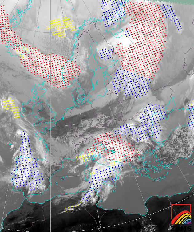
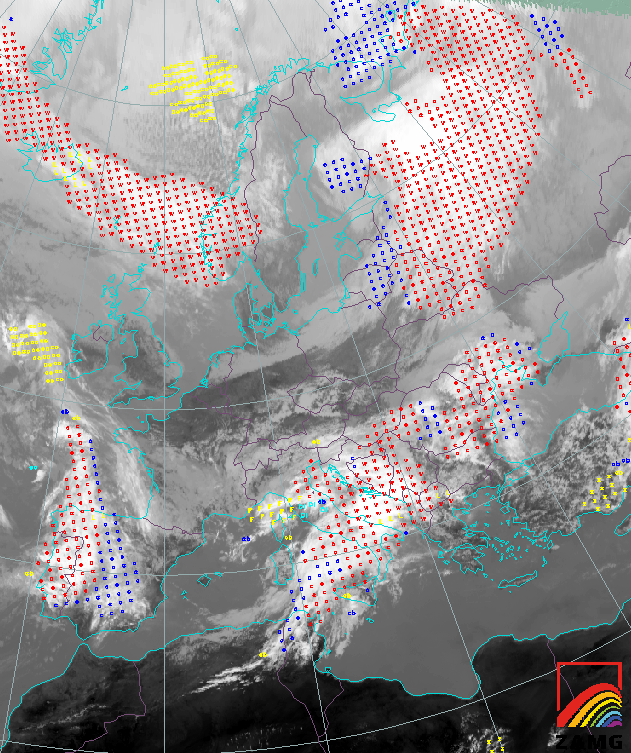
The chosen example shows ASII output for 28 March 2011 at 13:00 UTC.
- Visualisation of the ASII product (satellite information only):
Several frontal systems are detected, showing warm (red “w” tags) and cold fronts (blue “c” tags). Lee cloudiness has been detected over southern Italy (yellow “L” tags) and over Iceland. Two comma clouds (yellow “co” tags) were detected over the Arctic Sea and near Ireland.
- Visualisation of the ASIINWP product (including NWP fields):
The ASIINWP analysis shows similar results. Some deviations from the ASII analysis (i.e. without model fields) can nevertheless be observed. The cold front over Portugal is under warm air advection (red “c” tags), the same holds for the cold front between Tunisia and Italy.
For a complete list of the symbols used in the Figures see table 2.
Click on thumbnail for full-sized image
Figure 1: IR satellite image from 28th March 2011, 13 UTC, superimposed by the corresponding ASII product.
Click on thumbnail for full-sized image
Figure 2: IR satellite image from 28th March 2011, 13 UTC, superimposed by the corresponding ASIINWP product.
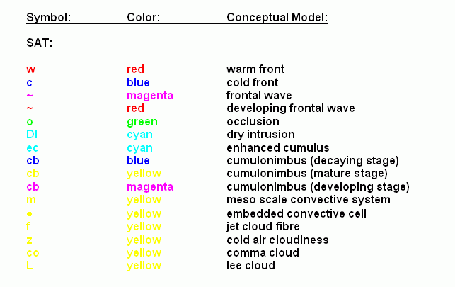
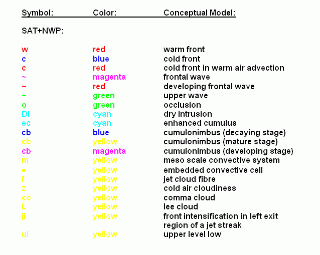
Table 2a and 2b: Symbols used for the visualisation of the ASII products.
2a: SAT: IR and WV satellite image as sole input
2b: SAT+NWP: NWP fields are added to the satellite image data